Differential analysis with HTSet

library(ggplot2)
library(knitr)
library(kableExtra)
library(dplyr)
library(HTSet)

introduction

High through-put experiments such as RNA-seq, proteomics, and metaboliomics estimate the abundance/concentration of hundrands to millions of features. Very commonly, researchers would like to answer questions such as which gene (or protein, metabolites) were differentially expressed or have differential abundance in treatment groups. Linear model and generalized linear model are widely used because they are highly flaxible to be adopted to different study designs. The HTSet package has a wrapper function model_fit() of three popular bioconductor packages, including limma, edgeR, and DESeq2, that performs differnetial analysis on a high through-put experiment dataset, and it returns the result in an organized structure.

The basic usage of model_fit() is below.

model_fit(object, design, coef, engine, args)

object must be a HTSet object. design is the study design matrix, usually returned by the model.matrix function. coef is the coefficient to perform statistical test. engine must be one of the three backend statistical package mentioned above. args is a list of additional parameters to be parsed to the backend statistical engine.

model_fit returns a list-like object. The elemenets that it contains are listed below.

results: A data.frame of the statistical test results for each gene/feature in each row. It has 5 columns. logFC has the estimate of the log2-fold-change corresponding to the effect. mean has the average lo2-expression for the gene/feature accross all samples. This is the AveExpr column in limma’s topTable or baseMean in DESeq2’s results. stat is the statistic value of the corresponding test. When using limma, this is the t-statistic value, same as the t column in the result of topTable. For edgeR, this is the f-statistic value for Quansi-likelihood test or the likelihood ratio statistic value for likelihood ratio test. Same as the column F or RT in the result of edgeR’s topTags. As for DESeq2, this is the Wald statistic value for Wald test or the difference in deviance between the reduced model and the full model for likelihood ratio test. same as the stat column in the output of DESeq2’s results. pval is the raw o-value and padj is the p-value after correction for multiple testing.
adjust.method: The method used to correct for multiple testing.
design: The design matrix
df: Degree of freedom for each gene/feature.
distribution: The distribution which the stat column in results is compared to generate the pval. This is t for t distribution for limma or DESeq2 with Wald test when useT eqauls to TRUE, f for f distribution for Quansi-likelihood test with edgeR, chisq for chi-squared distribution for likelihood ratio test with edgeR or DESeq2, and norm for DESeq2 with Wald test when useT equals to FALSE.
engin: The statistical package used as backend engine.
coef: The coefficient tested
params: Additional parameters parsed to model_fit

The HTSet package has two dataset included. They both can be loaded using the data() function.

data(exrna)
data(lipidome)

In this vignette, we will go though some examples of using model_fit() to perform statistical analysis with the two datasets.

Backend engines

count data

High through-put experimental data generated by nucleiic acid sequencing are were usually presented as counts per gene (RNA-seq) or counts per ASV/OTU (16S-seq). Counts data by nature do not fit gaussian distribution, thus linear model is not directly applicable. Thus, the major approches are (1) transforming counts data to continous data and normalized it, and (2) use negative binomial generalized linear model (glm). For the former approch, counts data are often transformed into logCPM followed by linear modeling. Another or a better approach is using limma’s voom function, which estimates the mean-variance relationship of the log-counts, and generates a precision weight for each observation. As for negative binomial glm, edgeR and DESeq2 two widely recognized packages.

exrna

The dataset exrna is the small RNA-seq result of isolated HDL from human plasma of 3 patients with systemic lupus erythematosus and 3 healthy control. The raw sequence fastq files were downloaded from GEO (GSE121865), and processed using the exceRNApipeline, using STAR agaist hg38. Gene counts were generated using htseq-count agaist gencode’s annotation.

exrna
#> S4 class: HTSet
#>   nsamples: 6    nfeatures:1084
#>   sample vars: 28    features vars: 2
#> slots:
#>   $edata: 1084x6 matrix
#>   $fdata: 1084x2 data.frame
#>   $pdata: 6x28 data.frame
#>   $assay: 0 list

kable(exrna$pdata[,c(1,2,4,7)], format = "html") %>%
    kable_styling()%>%
    column_spec(5, background = "orange") %>%
    scroll_box(width = "100%")

	anatomical_location	Assay.Type	BioProject	Condition
SRR8114380	High density lipoprotein	ncRNA-Seq	PRJNA498678	Systemic Lupus Erythematosus
SRR8114381	High density lipoprotein	ncRNA-Seq	PRJNA498678	Healthy Control
SRR8114382	High density lipoprotein	ncRNA-Seq	PRJNA498678	Systemic Lupus Erythematosus
SRR8114383	High density lipoprotein	ncRNA-Seq	PRJNA498678	Healthy Control
SRR8114384	High density lipoprotein	ncRNA-Seq	PRJNA498678	Systemic Lupus Erythematosus
SRR8114385	High density lipoprotein	ncRNA-Seq	PRJNA498678	Healthy Control

limma voom

We first create a study design matrix using the model.matrix function.

# create the design matrix
design = model.matrix( ~ Condition, data = exrna$pdata)
kable(design)

	(Intercept)	ConditionSystemic Lupus Erythematosus
SRR8114380	1	1
SRR8114381	1	0
SRR8114382	1	1
SRR8114383	1	0
SRR8114384	1	1
SRR8114385	1	0

We are going to test whether each gene is expressed differently between patinets and control, thus the cofficient that we are going to test should be ConditionSystemic Lupus Erythematosus (second column name). We can than call model_fit. Setting voom = TRUE tells model_fit to run voom before calling limma’s lmFit function.

coef = "ConditionSystemic Lupus Erythematosus"
fit1 = model_fit(exrna, design = design, coef = coef, engine = "limma", args = list(voom = TRUE))
#> Loading required namespace: limma
#> Loading required namespace: edgeR

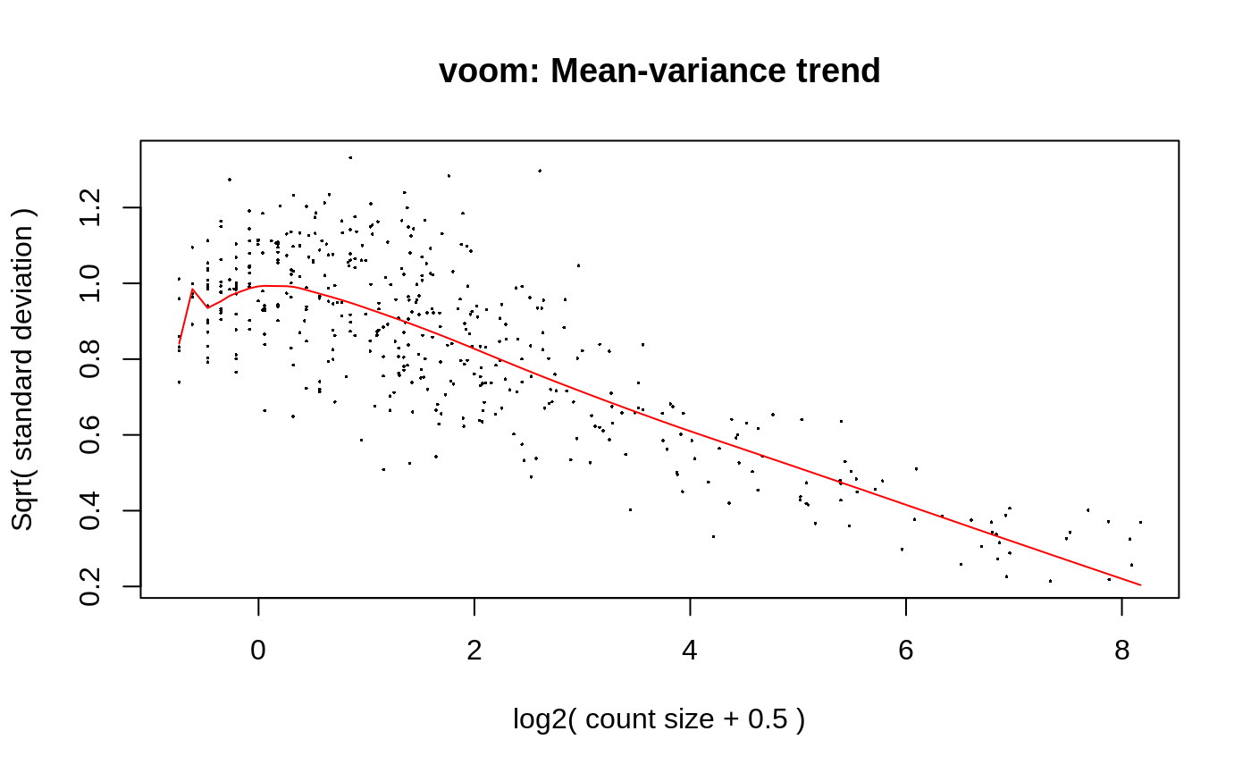
When args has an element named voom, model_fit calls the three functions voom, lmFit and eBayes in order. Additional arguments can be parsed to each of the three functions by assigning a list as value to the key of the corresponding step. For example, voom’s mean-variance trend plot was disabled by default. To enable the plot, parse it in a list to voom, as shown below.

fit1_2 = model_fit(exrna, design = design, coef = coef, engine = "limma",
                   args = list(voom = list(plot = TRUE)))

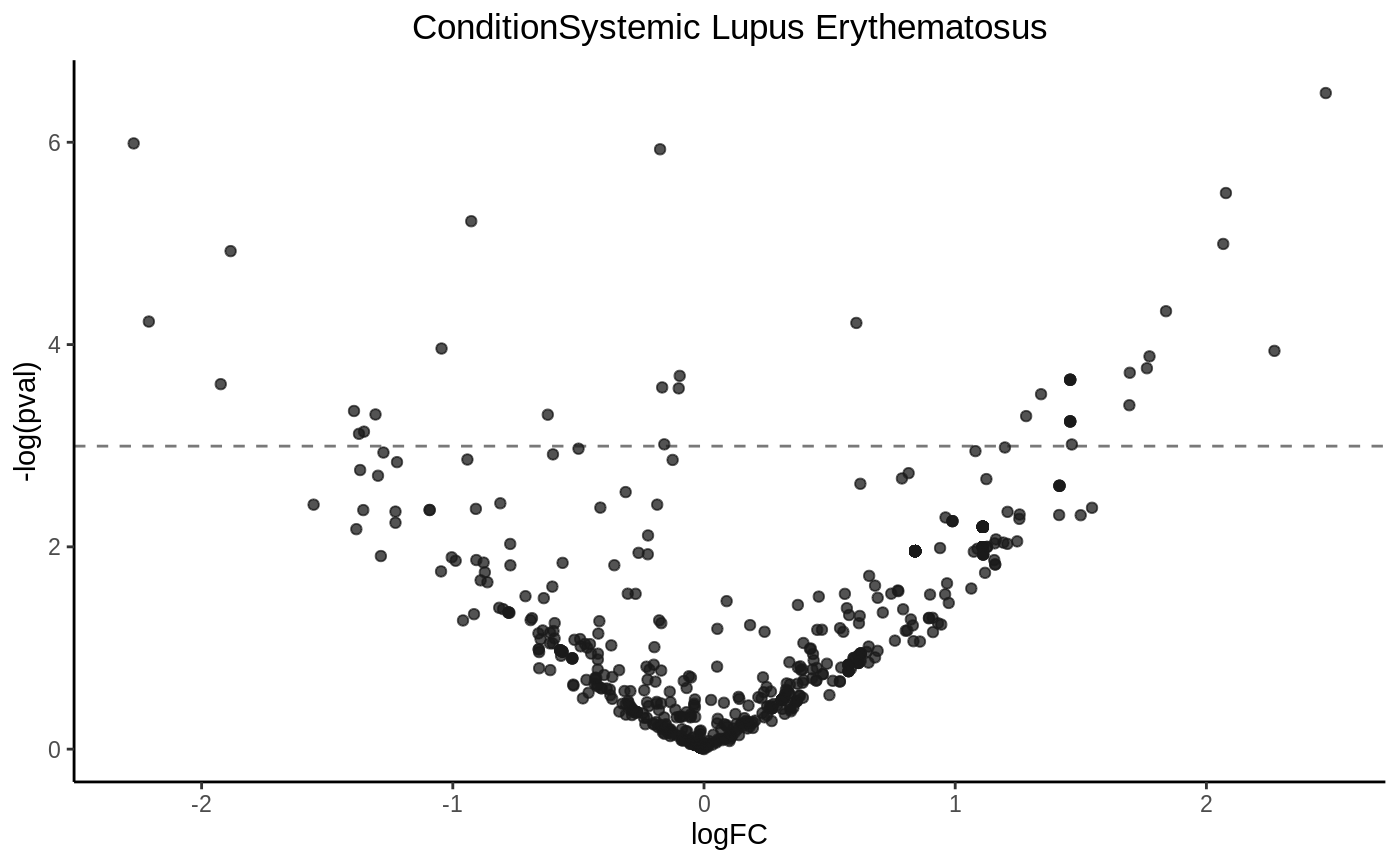
Draw a volcano plot

volcanoplot(fit1, hline = 0.05)

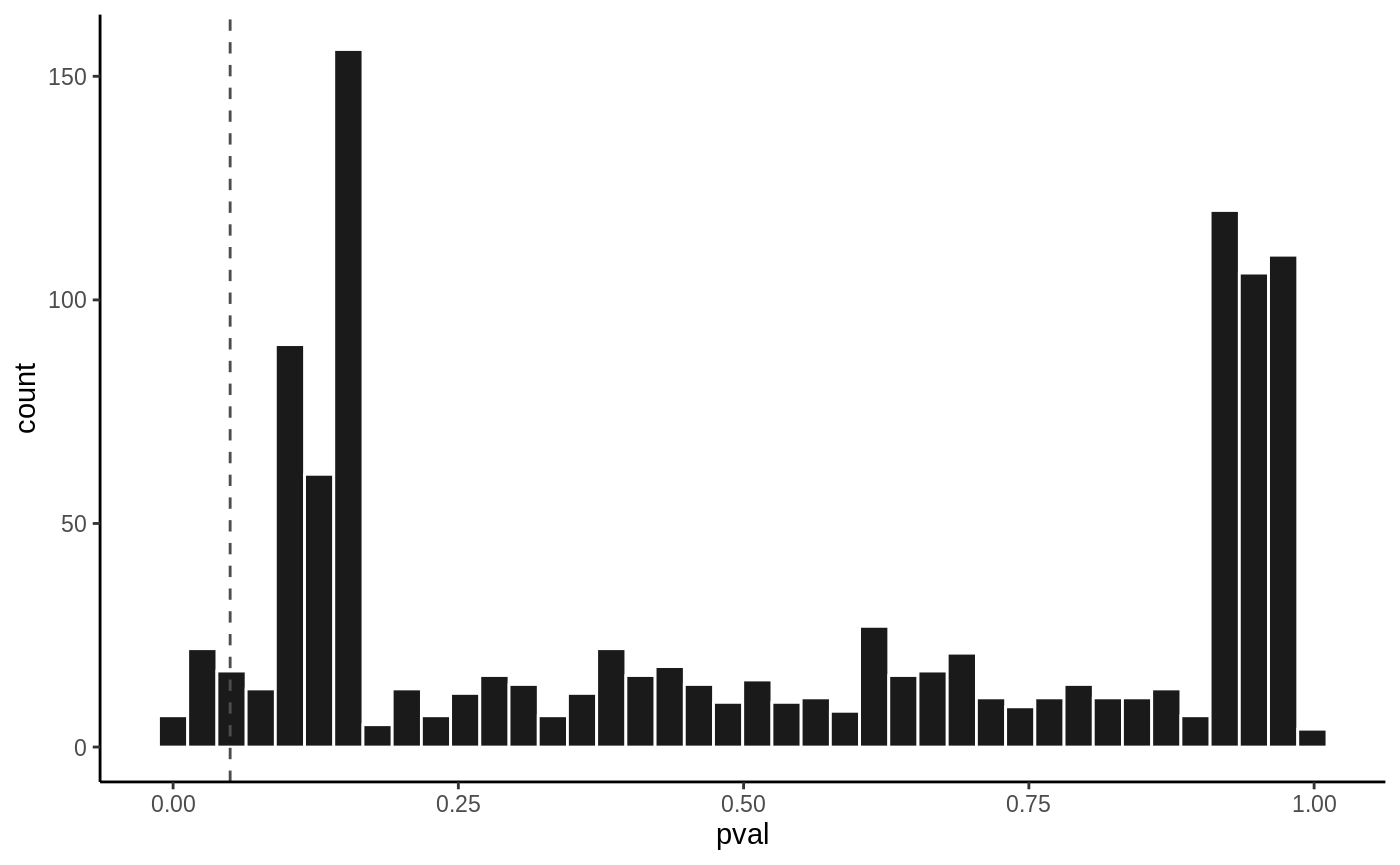
P value histogram

hist(fit1, vline = 0.05)

limma (but not voom)

It is also possible to transform count data into logCPM, and use limma directly.

exrna_cpm = exrna
exrna_cpm$edata = edgeR::cpm(exrna_cpm$edata, prior.count = 1, log = TRUE)
fit2 = model_fit(exrna_cpm, design = design, coef = coef, engine = "limma")

fit2$results[order(fit2$results$pval),] %>% head %>% kable()

	logFC	mean	stat	pval	padj
ENSG00000103769.10	-2.178666	8.969559	-4.596506	0.0004068	0.3260259
ENSG00000113319.13	1.578095	8.107325	4.240689	0.0008088	0.3260259
ENSG00000180210.14	-1.739524	8.624469	-4.184622	0.0009023	0.3260259
ENSG00000232807.2	1.382317	8.313330	3.643572	0.0026263	0.6277762
ENSG00000231662.1	-1.215158	8.191969	-3.327182	0.0049367	0.6277762
ENSG00000199804.1	1.170598	7.903577	3.324218	0.0049660	0.6277762

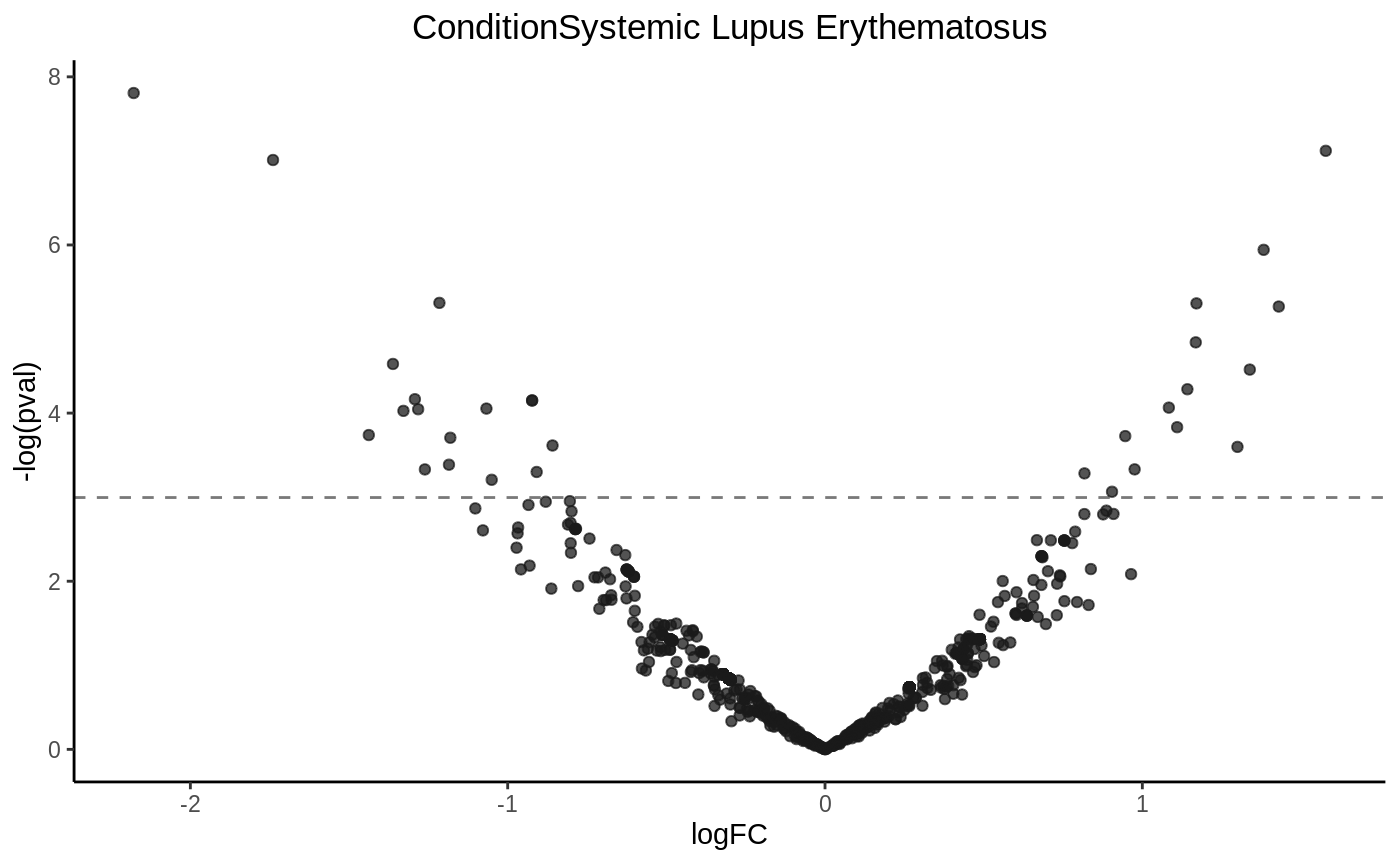
Drawing a volcano plot

volcanoplot(fit2, hline = 0.05)

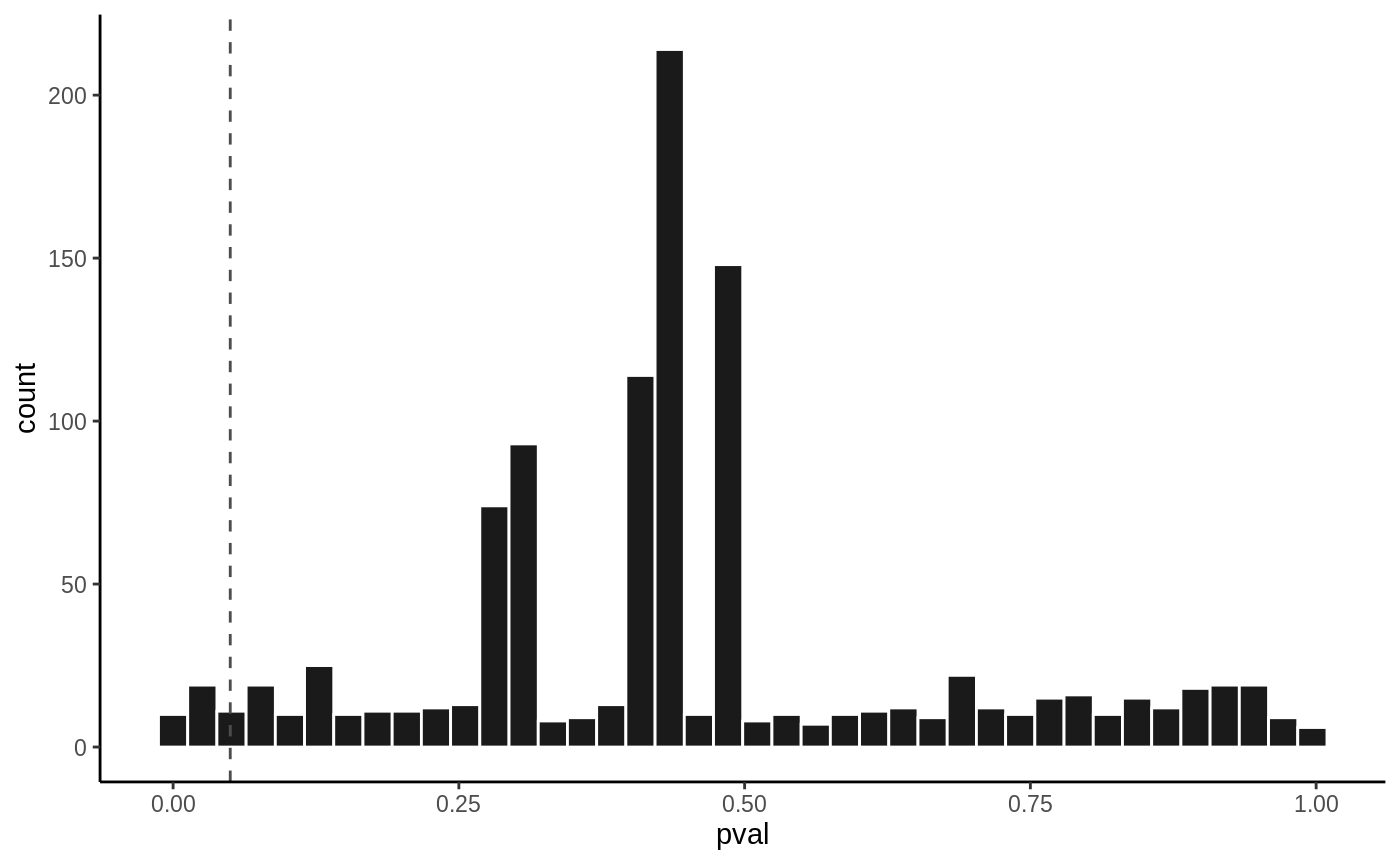
P value histogram

hist(fit2, vline = 0.05)

DESeq2

To use DESeq2 to perform negative binomial glm, simply set engine = "DESeq2"

fit3 = model_fit(exrna, design = design, coef = coef, engine = "DESeq2")
#> Loading required namespace: DESeq2
#> using supplied model matrix
#> estimating size factors
#> estimating dispersions
#> gene-wise dispersion estimates
#> mean-dispersion relationship
#> -- note: fitType='parametric', but the dispersion trend was not well captured by the
#>    function: y = a/x + b, and a local regression fit was automatically substituted.
#>    specify fitType='local' or 'mean' to avoid this message next time.
#> final dispersion estimates
#> fitting model and testing

Additional parameters can be parsed to the args as a list named as DESeq. The parameters will be used internally by the DESeq function. Use ?DESeq to see all parameters that can be used. For example, to use t distribution to estimate p-values:

fit3_2 = model_fit(
    exrna, design = design, coef = coef, engin = "DESeq2",
    args = list(
        DESeq = list(useT = TRUE)
    )
)
#> using supplied model matrix
#> estimating size factors
#> estimating dispersions
#> gene-wise dispersion estimates
#> mean-dispersion relationship
#> -- note: fitType='parametric', but the dispersion trend was not well captured by the
#>    function: y = a/x + b, and a local regression fit was automatically substituted.
#>    specify fitType='local' or 'mean' to avoid this message next time.
#> final dispersion estimates
#> fitting model and testing

DESeq2 also provides a likelihood ratio test. That can be done in a very similar way, by parsing additional arguments to the args parameter.

reduced = model.matrix(~1, data = exrna$pdata)
fit3_2 = model_fit(
    exrna, design = design, coef = coef, engin = "DESeq2",
    args = list(
        DESeq = list(test = "LRT", reduced = reduced)
    )
)
#> using supplied model matrix
#> estimating size factors
#> estimating dispersions
#> gene-wise dispersion estimates
#> mean-dispersion relationship
#> -- note: fitType='parametric', but the dispersion trend was not well captured by the
#>    function: y = a/x + b, and a local regression fit was automatically substituted.
#>    specify fitType='local' or 'mean' to avoid this message next time.
#> final dispersion estimates
#> fitting model and testing

fit3$results[order(fit3$results$pval),] %>% head %>% kable()

	logFC	mean	stat	pval	padj
ENSG00000103769.10	-2.5362785	3.178039	-2.187611	0.0286980	0.961832
ENSG00000207757.1	0.6388898	27.456948	2.098345	0.0358747	0.961832
ENSG00000210077.1	-0.9371747	11.433017	-1.793000	0.0729729	0.961832
ENSG00000113319.13	3.6485139	1.007428	1.623776	0.1044235	0.961832
ENSG00000008300.17	-1.4801477	4.102517	-1.623719	0.1044357	0.961832
ENSG00000116016.14	-2.7431868	1.681584	-1.614479	0.1064236	0.961832

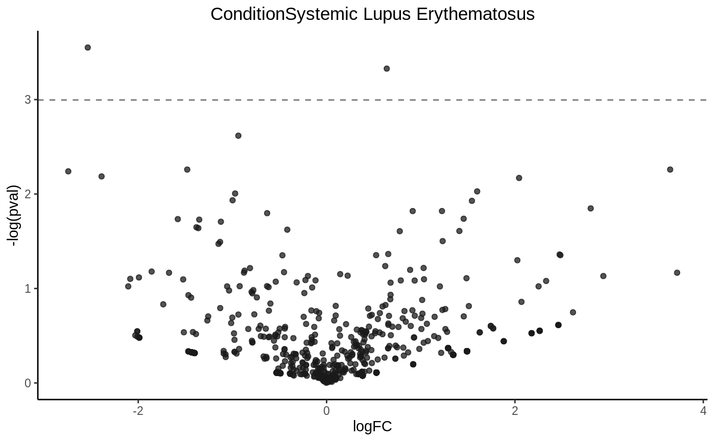
Drawing a volcano plot

volcanoplot(fit3, hline = 0.05)

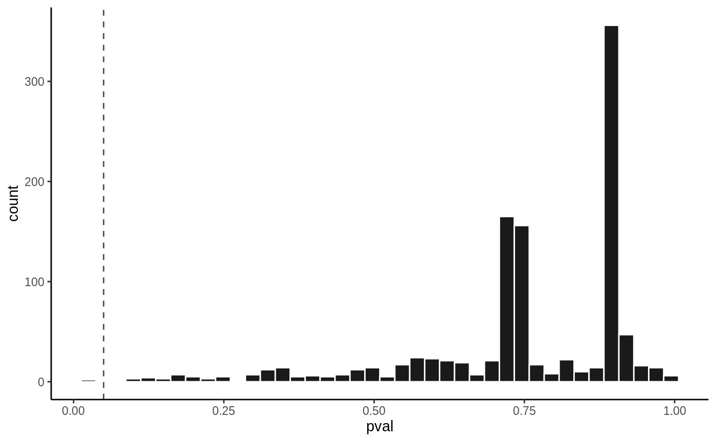
P value histogram

hist(fit3, vline = 0.05)

edgeR

Similar to DESeq2, edgeR also performes negative binomial glm test. Two models are provided by edgeR, the quasi-likelihood test (QLF) and likelihood ratio test (LRT). model_fit uses QLF by default.

fit4 = model_fit(exrna, design = design, coef = coef, engine = "edgeR")
fit4$results[order(fit4$results$pval),] %>% head %>% kable()

	logFC	mean	stat	pval	padj
ENSG00000103769.10	-2.3437702	9.869924	8.578464	0.0034193	0.5948105
ENSG00000210077.1	-0.9731867	11.183599	7.212137	0.0072688	0.5948105
ENSG00000207757.1	0.5768948	12.224554	7.091641	0.0095773	0.5948105
ENSG00000113319.13	3.9807611	8.828158	6.018755	0.0141937	0.5948105
ENSG00000116016.14	-2.6752084	9.264238	5.501202	0.0190482	0.5948105
ENSG00000008300.17	-1.6149331	9.950162	5.001152	0.0253811	0.5948105

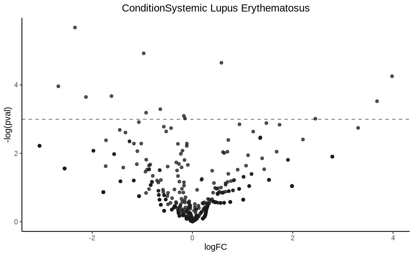
Drawing a volcano plot

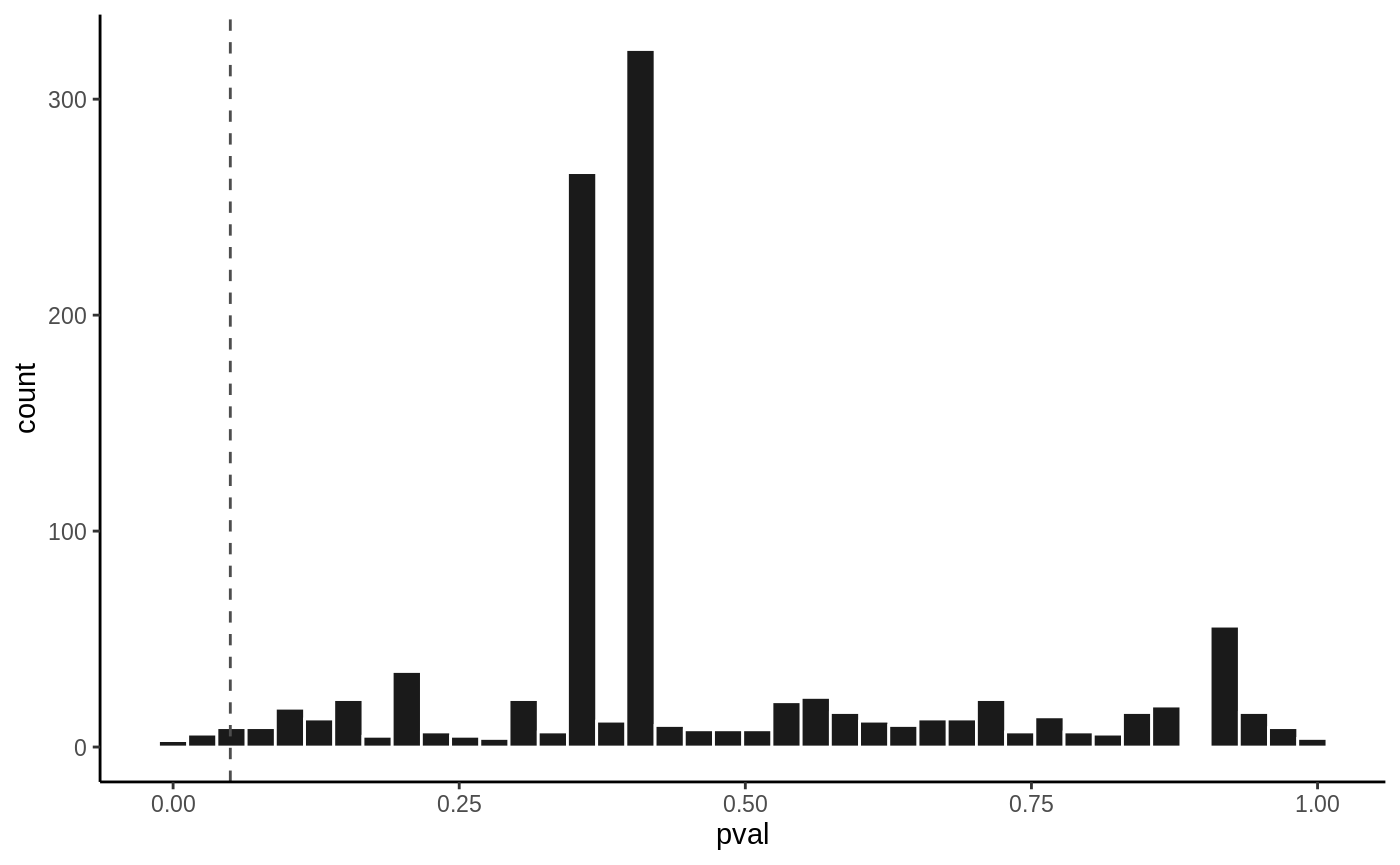
volcanoplot(fit4, hline = 0.05)

P value histogram

hist(fit4, vline = 0.05)

To use LRT, you need to specify it in the args.

fit5 = model_fit(exrna, design = design, coef = coef, engine = "edgeR",
                 args = list(model = "lrt"))
fit5$results[order(fit5$results$pval),] %>% head %>% kable()

	logFC	mean	stat	pval	padj
ENSG00000103769.10	-2.3437702	9.869924	9.981416	0.0015813	0.4090667
ENSG00000113319.13	3.9807611	8.828158	7.966385	0.0047654	0.4090667
ENSG00000210077.1	-0.9731867	11.183599	7.378458	0.0066010	0.4090667
ENSG00000116016.14	-2.6752084	9.264238	6.876766	0.0087323	0.4090667
ENSG00000207757.1	0.5768948	12.224554	6.693561	0.0096762	0.4090667
ENSG00000163631.17	3.6815563	8.740720	6.373366	0.0115846	0.4090667

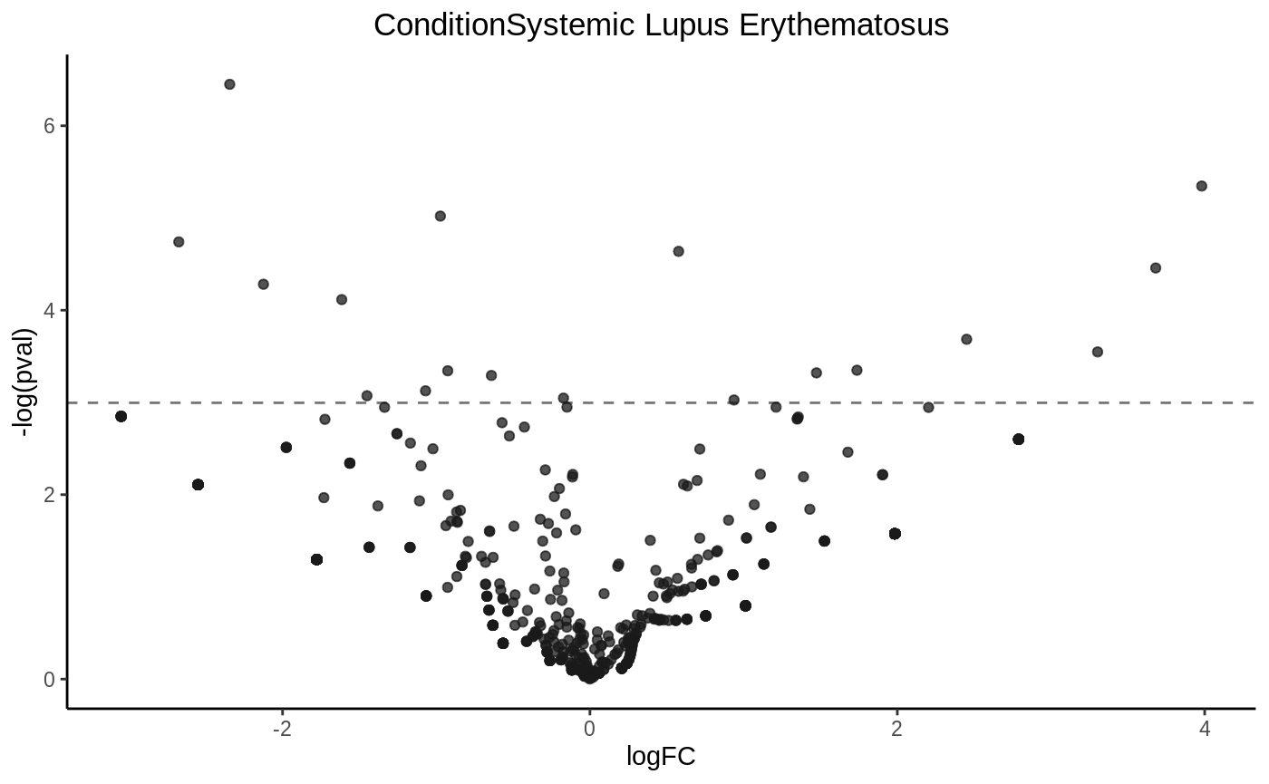
Drawing a volcano plot

volcanoplot(fit5, hline = 0.05)

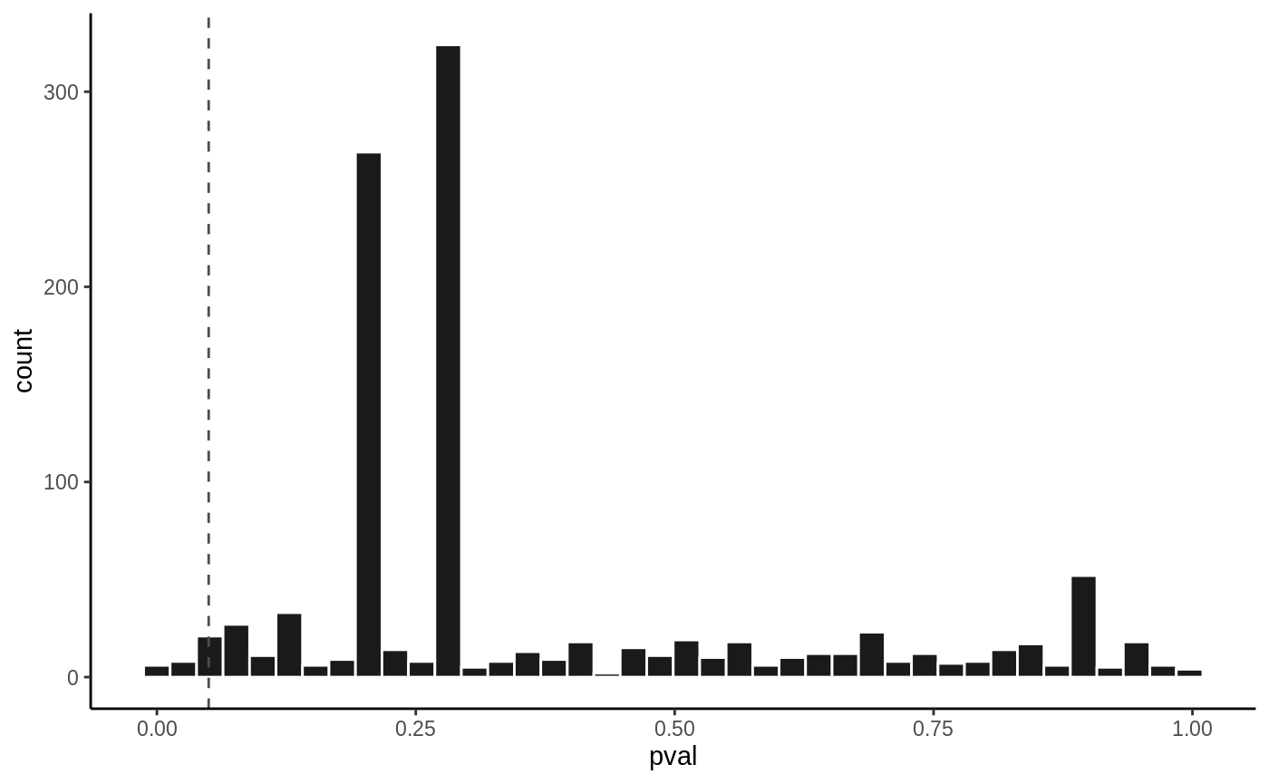
P value histogram

hist(fit5, vline = 0.05)

Complex models

lipidome

model_fit() also supports more complex study design models. The dataset lipidome is the result of a lipidomics analysis on isolated HDL from 10 human subjects in a 2x2 randomized cross-over study. The study was published on Metabolomics, 2019 (doi: 10.1007/s11306-019-1579-1).

lipidome
#> S4 class: HTSet
#>   nsamples: 40   nfeatures:170
#>   sample vars: 8 features vars: 15
#> slots:
#>   $edata: 170x40 matrix
#>   $fdata: 170x15 data.frame
#>   $pdata: 40x8 data.frame
#>   $assay: 0 list

summary(lipidome$pdata[,c("Treatment", "Timepoint")])
#>  Treatment Timepoint
#>  FF :20    Post:20  
#>  Med:20    Pre :20

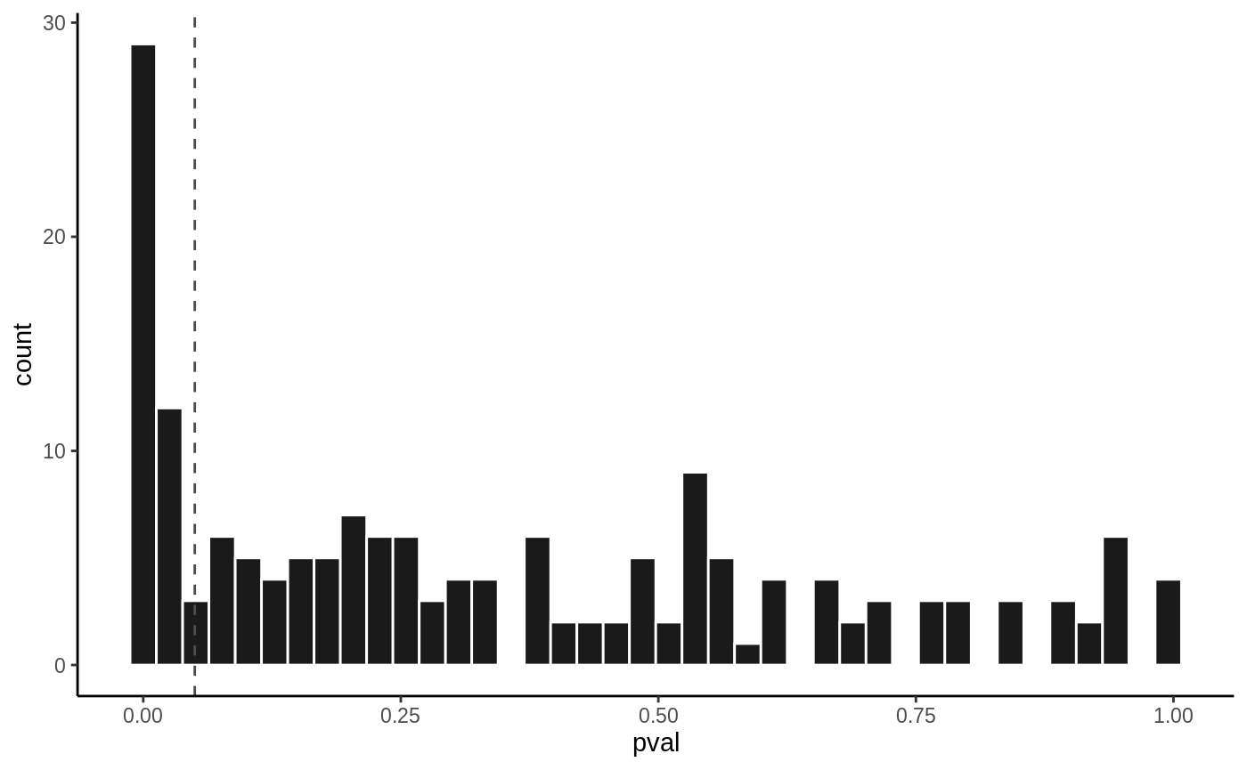
In the examples above, we were simply comparing disease patients to control. However in this study, we are asking a slightly more complex question. We would like to see how each lipid species change before and after the two treatments FF and Med. And since each subject was sampled four times, the model that we are using would be as blew. And \(\beta_3\) is the coefficient that we would like to test.

\[y = \beta_0 + \beta_1 Treatment + \beta_2 Timepoint + \beta_3 Timepoint*Treatment + \beta_4 Subject + e\]

The design matrix should be as below.

# in R's equation, ~ Treatment * Timepoint is a shorthand for 
# ~ Treatment + Timepoint + Treatment * Timepoint
design = model.matrix(~ Treatment * Timepoint + Subject + 1, data = lipidome$pdata)
coef = "TreatmentMed:TimepointPre"

Because the lipidome is continous data, the limma can be directly applied.

lipidome2 = transform_by_sample(lipidome, function(x) log(x/sum(x)))
fit6 = model_fit(lipidome2, design = design, coef = coef, engine = "limma")
fit6$results[order(fit6$results$pval),] %>% head %>% kable

	logFC	mean	stat	pval	padj
PC 36:2 p 1	0.9154783	-8.144336	5.495343	0.0000029	0.0004968
PC 34:2 p 1	0.7227051	-6.497471	4.730082	0.0000316	0.0018875
PC 38:4 p 2	0.4676405	-7.948502	4.713055	0.0000333	0.0018875
PC 35:2 1	0.5140877	-6.833362	4.583482	0.0000496	0.0021068
PE 38:4 p	0.7617776	-5.707228	4.326125	0.0001084	0.0030950
PC 34:2 p	0.6198772	-6.737366	4.323611	0.0001092	0.0030950

volcanoplot(fit6, hline = 0.05)

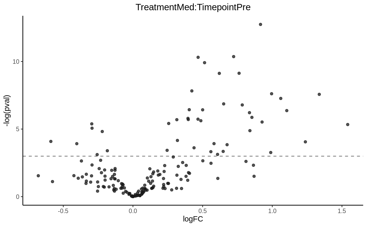
hist(fit6, vline = 0.05)

The End

model_fit() is simply a wrapper for the statistical pipelines from limma, edgeR, and DESeq2 with a clean interface and output format. You can certainly use limma, edgeR or DESeq2 directly and it is also not too complicated. Sometimes different models may come up with slightly different gene/feature list, however, as long as the model is approciate for the type of data to answer the specific question, your conclusion should be affected much. On thing to bear in mind that although most high through-put experiments are exploratory and hypothesis generating, running all different kinds of models and keep the one with the gene list that you like the most is probably a bad practice and may lead to inappropriate conclusion.

Chenghao Zhu

introduction

Backend engines

count data

exrna

limma voom

limma (but not voom)

DESeq2

edgeR

Complex models

lipidome

The End